Blogs/Manufacturing insights
The QRM Response Time Spiral: why long lead times create even longer lead times
Long manufacturing lead times encourage earlier release, more WIP, larger batches, and expediting — which grow queues and stretch lead time again.
Trooba Team
Long manufacturing lead times often create the very behaviours that make lead times longer. When delivery becomes unreliable, manufacturers release work earlier, increase buffers, expedite urgent orders, and build larger batches. Those actions increase work in process, variability, and congestion. Queues grow. Lead times stretch again.
This reinforcing cycle is what Quick Response Manufacturing describes as the QRM Response Time Spiral. Trooba Flow, our Factory Flow Intelligence software, approaches the same problem by modelling products, routings, resources, demand, and variability as a queueing network so manufacturers can see what is actually driving queue time, WIP, utilisation, and manufacturing lead time.
What is the QRM Response Time Spiral?
The QRM Response Time Spiral is a feedback loop in which long or unreliable response times encourage operating practices that create even more delay. A plant sees that orders are taking too long. Management responds by adding protection:
The Response Time Spiral · each protection step feeds the next
01
Unreliable lead time
02
Release earlier
03
WIP and queues grow
04
Expedite and interrupt
05
Add more protection
The loop returns to step 01: lead time is now even less reliable.
Each decision can look reasonable when viewed separately. Together, they can make factory flow worse. More work is released into the system. More jobs compete for the same machines and people. Expedites interrupt existing sequences. Batches hold downstream operations waiting. Utilisation rises. The result is more queueing. The plant now needs even more protection against unreliable lead times, and the spiral continues. For the broader strategy, see what Quick Response Manufacturing (QRM) is.
How long lead times create more WIP
One of the easiest ways to understand the spiral is through Little's Law:
WIP means work in process: all jobs that have entered the manufacturing system but have not yet finished. Suppose a factory completes 100 orders per week. If average manufacturing lead time is two weeks: WIP = 100 × 2 = 200 orders.
Now imagine deliveries become unreliable. Planners start releasing orders one week earlier so production has more time to complete them. If average time inside the system rises to three weeks while throughput remains 100 orders per week: WIP = 100 × 3 = 300 orders.
Little's Law at 100 orders per week · earlier release raises WIP
That additional work does not disappear. It waits in front of equipment. It sits between operations. It occupies floor space. It competes for labour and material handling. Planners spend more time deciding which order should move next. The extra protection intended to improve delivery performance can therefore increase the congestion causing poor delivery performance in the first place.
This is an illustrative example, not a measured customer result. Its purpose is to show the relationship described by Little's Law.
Why more WIP usually means more waiting
Manufacturing lead time is not simply processing time. A component might require only a few hours of actual machining, printing, assembly, or inspection while spending several days waiting between operations. That waiting occurs because resources are shared. When several jobs need the same machine, only one can usually be processed at a time. The rest form a queue.
Queueing theory tells us that waiting becomes increasingly sensitive as utilisation rises, particularly when arrivals and processing times vary. This is the practical message behind relationships such as Kingman's formula and other queueing approximations: queue time does not normally increase in a simple straight line as a resource approaches full utilisation. It can rise sharply.
That is why a factory can appear productive while customer lead time deteriorates. A machine running continuously may look efficient locally. But if the result is a large queue waiting in front of that machine, the factory as a whole may be slower. See why high utilisation increases lead time.
The five steps of the Response Time Spiral
The exact sequence differs between factories, but the underlying mechanism often looks like this.
01
Lead times become unreliable
Orders regularly take longer than expected. The instinctive response is to give production more time.
02
Work is released earlier
Planners launch jobs well before they are actually required at the first operation. The order is technically “in production,” but much of that additional time may be spent waiting. WIP increases.
03
Queues increase
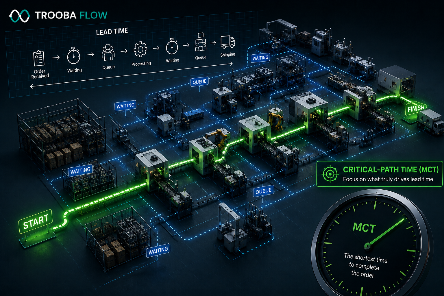
More jobs now compete for the same capacity. Even resources that were previously manageable can develop long queues when utilisation, variability, and WIP interact. Manufacturing Critical-Path Time (MCT) starts to grow.
04
Expediting increases
Some customer orders cannot tolerate the longer lead time. They become rush jobs. Rush jobs jump queues, change priorities, and disrupt established sequences. Jobs that were previously on time can now become late. Schedule variability increases.
05
More protection is added
Because the system has become less predictable, planners release future orders even earlier or add larger buffers. The loop begins again.
The Response Time Spiral is therefore not simply a scheduling problem. It is a system behaviour.
Why high utilisation can accelerate the spiral
A common response to poor performance is to push resources harder. If orders are late, managers naturally ask: “Why isn't this machine running?” That question makes sense when equipment is extremely expensive or genuine capacity shortages exist.
But maximising utilisation across every resource can create a different problem. A resource needs some spare capacity to absorb normal variability. Demand does not arrive perfectly evenly. Setup times change. Jobs take different amounts of time. Operators become unavailable. Rework happens. Material arrives late.
When a resource already operates close to its practical capacity, those fluctuations have nowhere to go. They become queues. This is why QRM often refers to strategic spare capacity. The objective is not idle equipment for its own sake. The objective is enough capacity flexibility to keep work moving quickly.
Batching can make the problem worse
Large batches are another common form of protection. The logic is understandable. If changing a machine takes time, run more pieces every time it is set up. That can reduce setup time per unit. But the local efficiency gain may create a system-level lead-time penalty.
Consider two operations. Operation A produces a batch of 500 pieces before sending it to Operation B. If Operation B cannot start until all 500 pieces are complete, the first finished piece waits while the remaining 499 are processed. Now consider transferring smaller quantities downstream while the larger production batch continues. Operation B can begin sooner.
Whole batch of 500 vs overlapping transfer lots
Wait for 500
Operation B cannot start until the full batch is complete
Transfer smaller lots
Operation B starts earlier while A continues on the rest
The processing time per individual part may not change at all. Yet manufacturing lead time can fall because waiting between operations is reduced. This distinction between production lot size and transfer lot size is important in flow improvement. Large batches can make machines look efficient while making orders move slowly.
The spiral changes management behaviour too
The Response Time Spiral is not only physical. It also creates administrative work. Long lead times often lead to more schedule meetings, more customer-status requests, more manual reprioritisation, more expediting, more buffer calculations, more forecast dependence, and more coordination between departments.
People begin managing exceptions instead of improving flow. Eventually the factory can reach a strange state: everyone is busy, machines are busy, planners are busy, yet orders continue to wait. That is one reason reducing lead time can produce benefits beyond faster delivery. A more responsive system can require less intervention simply to keep orders moving.
Common reactions versus flow-oriented responses
| When lead time increases | Common reaction | Possible flow effect | Flow-oriented question |
|---|---|---|---|
| Orders are late | Release work earlier | More WIP and queueing | Why are orders waiting? |
| Machine looks overloaded | Push utilisation higher | Longer queues | Is capacity or variability driving the queue? |
| Setups seem expensive | Increase batch sizes | More waiting between operations | Can lot or transfer sizes be reduced? |
| Customer order is urgent | Expedite it | Disrupts other jobs | Why is normal flow unreliable? |
| Delivery dates are missed | Add more safety time | Longer planned response time | What is driving MCT? |
The purpose is not to claim that every early release, large batch, or expedite is wrong. Sometimes these actions are necessary. The problem begins when they become permanent substitutes for understanding the underlying flow problem.
How to break the QRM Response Time Spiral
Breaking the spiral starts by changing the question. Instead of asking how we push more work through each machine, ask what is preventing orders from moving through the factory quickly. That requires separating processing time from waiting time.
For each important product family, examine:
The answer is often not “buy another machine.” It may be a routing change, capacity adjustment, smaller transfer lot, different product grouping, reduction in variability, or a change in how work is released. That is also where modelling can help.
Trooba Flow uses queueing theory, QRM principles, MCT, and factory-flow modelling to estimate how changes to resources, routings, shifts, or lot policies may affect queues and manufacturing lead time before those changes are made on the shop floor. The result of such an analysis is a modelled projection, not a measured outcome. Actual performance still needs to be verified after implementation.
A measured example of changing the flow instead of the machines
MEASURED RESULT — TARINIKA
Tarinika, a jewellery manufacturer, reduced manufacturing lead time using the same factory and the same machines. The constraint was lot sizing and queue dynamics, not machine speed.
That distinction matters. If the problem had been interpreted purely as insufficient machine capacity, the logical response might have been additional equipment. Instead, the improvement came from changing how work flowed through the existing system.
This is the central lesson of the Response Time Spiral. Long lead times should not automatically trigger more buffers, more WIP, larger batches, or higher utilisation. First understand why work is waiting.
See what is driving lead time in your factory.
Request a Flow AnalysisIn short
The QRM Response Time Spiral explains why manufacturing lead time can become self-reinforcing. Long lead times encourage manufacturers to release work earlier, increase WIP, batch more aggressively, and expedite more frequently. Those behaviours increase congestion and variability. Queues grow, which makes lead times longer and less predictable.
Breaking the spiral requires shifting attention from local efficiency to factory flow. Measure waiting. Understand utilisation. Study variability. Examine lot sizes. Identify the resources that actually control response time. Then test changes against the system as a whole.
If you want to identify what is driving lead time in your factory, you can request a Flow Analysis at trooba.com/flow-analysis.
FAQs
What is the QRM Response Time Spiral?
The QRM Response Time Spiral describes a reinforcing cycle where long manufacturing lead times encourage behaviours such as releasing work earlier, increasing buffers, batching, and expediting. These actions can increase WIP, variability, and queueing, which makes lead times even longer. Quick Response Manufacturing uses the concept to show why reducing response time often requires changing system policies, not simply working faster.
Why does releasing production orders earlier increase lead time?
Early release puts more work into the manufacturing system before capacity is ready to process it. The additional WIP competes for shared machines and labour, creating queues between operations. Releasing earlier may give an individual order more calendar time, but if it becomes standard practice across many orders, congestion can increase and overall manufacturing lead time can become longer.
Does high machine utilisation always cause long lead times?
No. High utilisation is not automatically bad, and some expensive or constrained resources need to operate at high utilisation. The risk appears when a resource has little spare capacity and faces meaningful variability. In that situation, normal fluctuations in arrivals or processing times can create disproportionately larger queues, increasing waiting time even if the machine itself is operating efficiently.
How is WIP connected to manufacturing lead time?
Little's Law connects WIP, throughput, and lead time: WIP = Throughput × Lead Time. At a stable throughput rate, longer lead times are associated with more work inside the system. This does not mean every reduction in WIP automatically fixes lead time, but it provides a useful way to understand why excessive early releases and congested queues often appear together.
How can a manufacturer tell whether capacity or queueing is causing long lead times?
Start by separating processing time from waiting time and examining utilisation, queue time, variability, and WIP by resource. A genuine capacity constraint will usually remain heavily loaded even after flow policies are examined. In other cases, long lead time may be driven primarily by variability, batching, routing interactions, or work-release policies rather than insufficient equipment.
See what is driving lead time in your factory.
Request a Flow Analysis